2  Data

New York City’s 311 system is how, residents let the city know about issues in their communities, such as noise, heating problems, trash, and illegal parking etc. Each entry in the 311 data represents a moment when someone was concerned enough to reach out to the city for assistance.

2.1 Data Source and Scope

The raw data come from the NYC Open Data 311 service request API. To avoid time-outs and memory issues, we chose to download the data month-by-month, combined, and then saved as an .rds file for efficient reuse. In total, the working dataset contains around 6M over a two-year window, from early 2023 through late 2024.

library(dplyr)
library(tidyr)
library(ggplot2)
library(stringr)
library(memoise)

# library(RSocrata)
# library(dplyr)

# options(timeout = 600)

# base_url <- "https://data.cityofnewyork.us/resource/erm2-nwe9.json"

# get_month_data <- function(year, month) {
#   start <- sprintf("%d-%02d-01T00:00:00", year, month)
#   # end = first day of next month
#   if (month == 12) {
#     end <- sprintf("%d-01-01T00:00:00", year + 1)
#   } else {
#     end <- sprintf("%d-%02d-01T00:00:00", year, month + 1)
#   }

#   url <- sprintf(
#     "%s?$where=created_date >= '%s' AND created_date < '%s'",
#     base_url, start, end
#   )
#   message("Fetching: ", start, " to ", end)
#   read.socrata(url)
# }

# # Example: all months of 2023
# months <- 1:12
# list_2023 <- lapply(months, function(m) get_month_data(2023, m))
# data_2023 <- bind_rows(list_2023)
# list_2024 <- lapply(months, function(m) get_month_data(2024, m))
# data_2024 <- bind_rows(list_2024)
# combined <- rbind(data_2023,data_2024)
# saveRDS(combined, "nyc_311_data.rds")

combined=combined <- readRDS("nyc_311_data.rds")
#combined=combined <- readRDS("nyc_311_data.rds")

Each row corresponds to a single 311 complaint and includes the following groups of variables:

2.1.1 Timestamps

• created_date: when the complaint was submitted
  
• closed_date: when the complaint was closed (if ever)
  
• resolution_action_updated_date: when a resolution action was logged

2.1.2 Categorical Descriptors

• agency, agency_name
  
• complaint_type and a higher-level complaint_bucket (custom grouping)
  
• descriptor (more detailed description of the issue)
  
• status (e.g., "Closed", "Assigned", "In Progress")

2.1.3 Location Information

• borough, incident_zip, incident_address
  
• location_type (e.g., "RESIDENTIAL BUILDING", "Street/Sidewalk")
  
• latitude, longitude

2.1.4 Channel and Resolution

• open_data_channel_type (e.g., ONLINE, PHONE, MOBILE, OTHER)
  
• resolution_description and resolution_action fields

2.2 Data Quality: Missingness Across Columns

Before doing any substantive analysis, we examined the completeness of the raw 311 dataset. The goal of this step was to understand which variables are reliable, which ones are mostly empty, and where cleaning or dropping variables is justified.

missing_values_summary <- colSums(is.na(combined))
missing_columns <- missing_values_summary[missing_values_summary > 0]
missing_table <- data.frame(
  Column = names(missing_columns),
  MissingCount = as.numeric(missing_columns)
)
sorted_table <- missing_table |>
arrange(desc(MissingCount))
print(sorted_table)

                           Column MissingCount
1            taxi_company_borough      6679852
2                       road_ramp      6668175
3        bridge_highway_direction      6660223
4                        due_date      6651779
5             bridge_highway_name      6639447
6          bridge_highway_segment      6639437
7           taxi_pick_up_location      6611318
8                    vehicle_type      6504338
9                   facility_type      6199357
10                       landmark      2652950
11          intersection_street_1      2180001
12          intersection_street_2      2176719
13                 cross_street_1      1903203
14                 cross_street_2      1902070
15                  location_type       800974
16                            bbl       752073
17                           city       325436
18                    street_name       244008
19               incident_address       243812
20                    closed_date       133656
21                       latitude       102706
22                      longitude       102706
23              location.latitude       102706
24             location.longitude       102706
25         location.human_address       102706
26       x_coordinate_state_plane       102597
27       y_coordinate_state_plane       101804
28         resolution_description        93259
29                     descriptor        78842
30                   incident_zip        72906
31 resolution_action_updated_date        37625
32                   address_type        30391
33                   created_date            1

library(dplyr)
library(tidyr)
library(ggplot2)
library(scales)

# 1) Compute missingness per column
miss_by_col_all <- combined |>
  summarise(across(everything(), \(x) sum(is.na(x)))) |>
  pivot_longer(everything(), names_to = "column", values_to = "missing_n") |>
  mutate(
    total_n      = nrow(combined),
    missing_rate = missing_n / total_n
  ) |>
  arrange(desc(missing_n))

# 2) Top 25 columns by missing rate, add index label
top_missing_rate <- miss_by_col_all |>
  slice_max(missing_rate, n = 25) |>
  arrange(desc(missing_rate)) |>
  mutate(
    rank_label = paste0(row_number(), ". ", column),
    rank_label = factor(rank_label, levels = rev(rank_label))  # for coord_flip
  )

# 3) Nice bar plot
p_missing <- ggplot(top_missing_rate,
                    aes(x = rank_label, y = missing_rate, fill = missing_rate)) +
  geom_col(width = 0.8) +
  coord_flip() +
  scale_y_continuous(
    labels = percent_format(accuracy = 1),
    expand = expansion(mult = c(0, 0.05))
  ) +
  scale_fill_viridis_c(
    option = "C",
    direction = -1,
    name = "Missing rate"
  ) +
  labs(
    title = "Top Columns by Missingness Rate",
    x = "Features",
    y = "Missingness rate"
  ) +
  theme_minimal(base_size = 13) +
  theme(
    panel.grid.minor = element_blank(),
    axis.text.y  = element_text(size = 9),
    axis.text.x  = element_text(size = 10),
    plot.title   = element_text(face = "bold", size = 16),
    plot.subtitle = element_text(size = 11),
    legend.position = "right"
  )

p_missing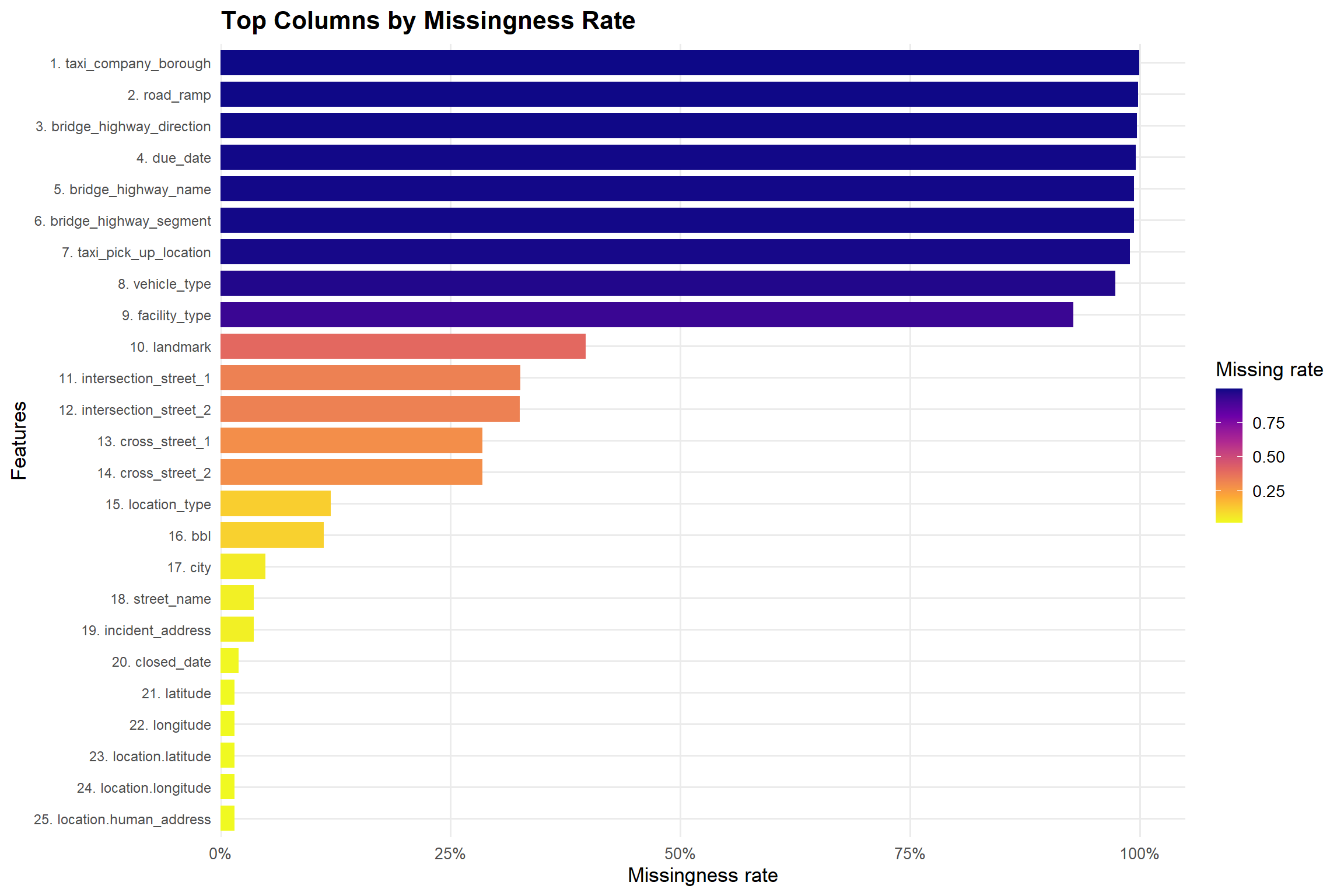

# 4) Threshold + list of columns to drop (same logic as before)
missing_threshold <- 0.60

cols_to_drop_by_missing <- miss_by_col_all |>
  filter(missing_rate > missing_threshold) |>
  pull(column)

The first plot shows the 25 columns with the highest proportion of missing values. Each bar is a column, ordered from most to least missing, and the color scale encodes the missingness rate.

Key observations:

• Several columns have almost complete missingness (≈ 95–100%), including
  taxi_company_borough, road_ramp, bridge_highway_direction, bridge_highway_name,
  bridge_highway_segment, and taxi_pick_up_location.
• Many of these fields are highly specialized (e.g., taxi or bridge/highway metadata) that apply only to a very small subset of 311 requests.
• A second tier of columns (e.g., intersection_street_1, intersection_street_2, cross_street_1, cross_street_2) has moderate missingness (roughly 25–40%), typically for records where complaints do not occur at an intersection. We decided to remove extreme missingness columns from final dataframe, which will add noise and complexity without contributing to the main objective of the project and columns with moderate missingness but high potential value were kept for further analysis.

set.seed(42)
sampled_data <- combined[sample(1:nrow(combined), 5000), ]

missing_long <- as.data.frame(is.na(sampled_data)) |>
  pivot_longer(cols = everything(), names_to = "Column", values_to = "IsMissing")

missing_long <- cbind(RowIndex = rep(1:nrow(sampled_data), times = ncol(sampled_data)), missing_long)

# Plotting heatmap of missing data
ggplot(missing_long, aes(x = Column, y = RowIndex, fill = IsMissing)) +
  geom_tile() +
  scale_fill_manual(values = c("FALSE" = "white", "TRUE" = "red"), name = "Missing") +
  labs(title = "Heatmap of Missing Data (Sampled Rows)",
       x = "Columns",
       y = "Row Index") +
  theme_minimal() +
  theme(axis.text.x = element_text(angle = 90, hjust = 1))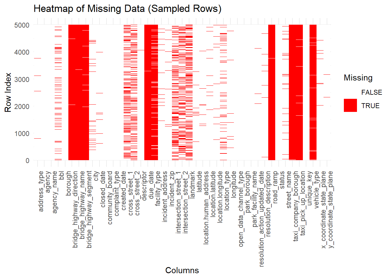

To complement the summary bar chart, we also visualized missingness row by row for a random sample of records. In this heatmap:

• Some columns form solid vertical red bands, meaning they are missing for almost all rows which correspond to the heavily missing taxi/bridge fields seen in the previous plot.
• Other columns show stripe-like patterns, where only some rows are missing (e.g., closed_date for still-open complaints).
• Core analytical fields such as created_date, complaint_type, and borough appear almost entirely white, confirming that they are reliable.

2.3 Focusing on Key Categorical Variables

library(dplyr)
library(ggplot2)
library(scales)


# Borough counts on cleaned data
borough_counts <- combined |>
  count(borough, name = "n") |>
  mutate(
    share = n / sum(n),
    label_text = paste0(comma(n), " (", percent(share, accuracy = 0.05), ")")
  ) |>
  arrange(desc(n))

ggplot(borough_counts,
       aes(x = reorder(borough, n), y = n)) +
  geom_col(width = 0.7, fill = "#1b9e77") +
  scale_y_continuous(
    labels = scales::comma,
    breaks = scales::pretty_breaks(n = 8),
    expand = expansion(mult = c(0, 0.15))
  ) +
  labs(
    title = "Borough Distribution of 311 Complaints",
    x = "NYC Borough",
    y = "Number of complaints"
  ) +
  theme_minimal(base_size = 13) +
  theme(
    panel.grid.minor = element_blank(),
    axis.text.y  = element_text(size = 10),
    axis.text.x  = element_text(size = 10),
    plot.title   = element_text(face = "bold", size = 16),
    plot.subtitle = element_text(size = 11),
    legend.position = "right"
  )

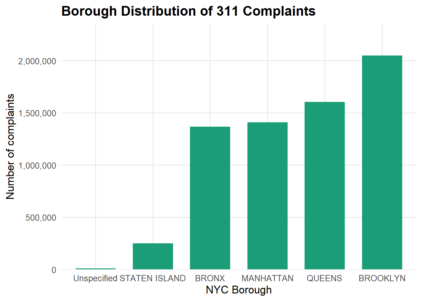
Interpretation:

• Unspecified boroughs ~ 8000 complaints (0.1%) were excluded in final data.
• Brooklyn and Queens together account for more than half of all 311 complaints, which is broadly consistent with their larger populations and geographic size.
• Staten Island contributes a comparatively small share of complaints (3.7%), reflecting both its smaller population and possibly different usage patterns of 311.

This plot acts as a sanity check that the dataset reflects known patterns of NYC population and service use and also it provides context for later plots that break down complaint types and system performance within each borough.

Missingness Pattern for Core Categorical Variables

#label
valid_boros <- c("MANHATTAN", "BROOKLYN", "QUEENS", "BRONX", "STATEN ISLAND")

df_clean_final <- combined |>
  filter(borough %in% valid_boros)

df_clean_final <- df_clean_final |>
  dplyr::select(
    unique_key, created_date, closed_date, resolution_action_updated_date,
    agency, agency_name, complaint_type, descriptor, status,
    borough, city, incident_zip, incident_address,
    latitude, longitude, location_type,
    open_data_channel_type,
    resolution_description
  )
#saveRDS(df_clean_final, "df_clean_final.rds")

combined0 <- combined |>
  mutate(
    across(where(is.character), \(x) str_squish(x)),
    across(where(is.character), \(x) na_if(x, ""))
  )

miss_by_col_all <- combined0 |>
  summarise(across(everything(), \(x) sum(is.na(x)))) |>
  pivot_longer(everything(), names_to = "column", values_to = "missing_n") |>
  mutate(total_n = nrow(combined0),
         missing_rate = missing_n / total_n) |>
  arrange(desc(missing_n))

library(dplyr)
library(stringr)
library(lubridate)

df0 <- df_clean_final |>
  mutate(
    across(where(is.character), \(x) str_squish(x)),
    across(where(is.character), \(x) na_if(x, "")),
    across(where(is.character), \(x) na_if(x, "NA")),
    across(where(is.character), \(x) na_if(x, "N/A"))
  )

library(redav)
critical_cols <- c("location_type", "complaint_type", "borough")
plot_missing(df0[critical_cols])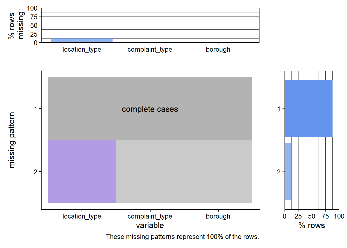

Main findings:

• borough and complaint_type are essentially complete almost no records are missing these fields.
• location_type has a small but noticeable amount of missingness (around 10–15% of rows). The plot shows two main patterns:
  1. Complete cases (all three variables present).
     
  2. Cases where only location_type is missing.
• For analyses that depend heavily on location_type (e.g., location-type heatmaps and action distributions), we restrict to complete cases so that percentages are meaningful.
• For other analyses, we kept "Unknown" or NA category for location_type, so that rows are not discarded unnecessarily.

2.4 Spatial Data Quality Checks

Many of the most interesting 311 questions are spatial (Which neighborhoods complain the most? Where are issues slowest to resolve?), so we checked the quality of the geographic fields before using them.

library(dplyr)
library(ggplot2)
library(scales)

# 1. Compute geolocation validity
geo_check <- df0 |>
  transmute(
    latitude = suppressWarnings(as.numeric(latitude)),
    longitude = suppressWarnings(as.numeric(longitude)),
    geo_ok = !is.na(latitude) & !is.na(longitude) &
      between(latitude, 40, 41.2) &
      between(longitude, -74.5, -73.2)
  )

# 2. Prepare summary for % view
geo_summary <- geo_check |>
  count(geo_ok) |>
  mutate(
    label = ifelse(geo_ok, "Valid NYC Coordinates", "Invalid / Missing Coordinates"),
    pct = n / sum(n)
  )

# 3. Plot
ggplot(geo_summary, aes(x = label, y = pct, fill = label)) +
  geom_col(width = 0.6, alpha = 0.85) +
  geom_text(aes(label = percent(pct, accuracy = 0.1)),
            vjust = -0.5, size = 5) +
  scale_y_continuous(labels = percent_format(accuracy = 1),
                     expand = expansion(mult = c(0, 0.1))) +
  scale_fill_manual(values = c("#1b9e77", "#d95f02")) +
  labs(
    title = "Geolocation Validity of 311 Records",
    x = "Geolocation Status",
    y = "% of Records",
    fill = NULL
  ) +
  theme_minimal(base_size = 14) +
  theme(
    legend.position = "none",
    plot.title = element_text(face = "bold")
  )

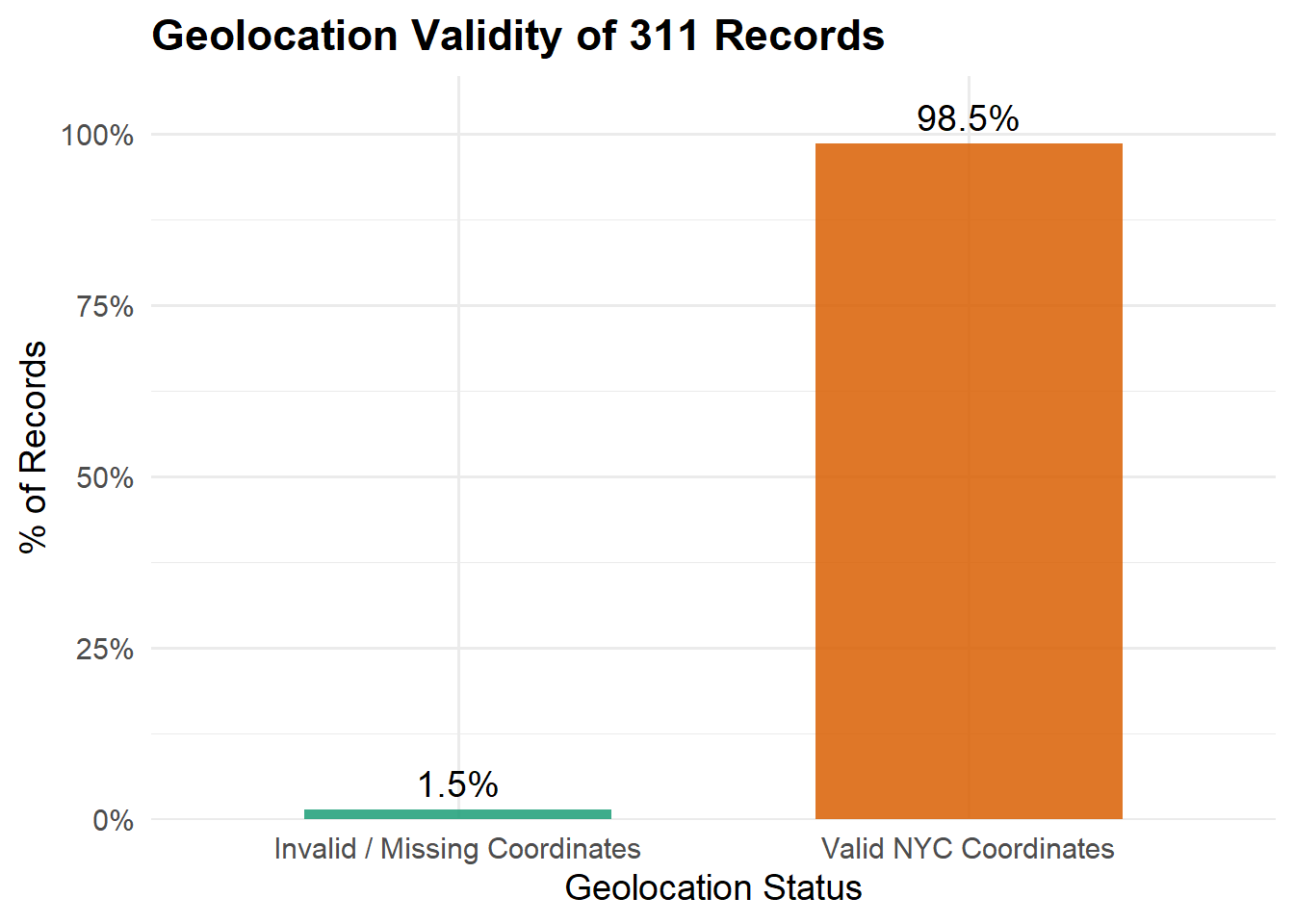
The bar chart shows:

• 98.5% of records have valid latitude–longitude pairs.Only 1.5% are invalid or missing.
  
• When making maps or location summaries, we’ll only use the valid coordinate subset. This prevented us from plotting points that are clearly wrong (like locations outside of NYC or at (0, 0)).

library(dplyr)
library(ggplot2)
library(scales)

df_zip <- df_clean_final |>
  mutate(
    zip_num = suppressWarnings(as.numeric(incident_zip)),
    zip_category = case_when(
      is.na(zip_num) ~ "Missing ZIP",
      zip_num >= 10000 & zip_num <= 11697 ~ "Valid NYC ZIP",
      TRUE ~ "Invalid ZIP"
    )
  ) |>
  count(zip_category) |>
  mutate(
    percent = n / sum(n),
    label = paste0(comma(n), " (", percent_format(accuracy = 0.1)(percent), ")")
  )

ggplot(df_zip, aes(x = reorder(zip_category, -n), y = n, fill = zip_category)) +
  geom_col(width = 0.6) +
  
  scale_fill_manual(values = c(
    "Valid NYC ZIP" = "#1b9e77",
    "Invalid ZIP"   = "#d95f02",
    "Missing ZIP"   = "#7570b3"
  )) +
  
  # FIX: expand limits so labels never get clipped or flipped
  scale_y_continuous(
    labels = comma,
    expand = expansion(mult = c(0, 0.15))  # extra 15% space above
  ) +
  
  labs(
    title = "ZIP Code Quality Summary",
    x = "Zip Code Category",
    y = "Number of Records"
  ) +
  
  theme_minimal(base_size = 13) +
  theme(
    legend.position = "none",
    plot.title = element_text(face = "bold", size = 18)
  )

df_clean <- df_clean_final %>%
  mutate(
    zip_num = suppressWarnings(as.numeric(incident_zip))
  ) %>%
  filter(
    !is.na(zip_num),
    zip_num >= 10000,
    zip_num <= 11697
  ) %>%
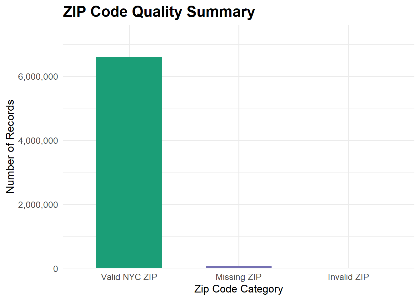
  select(-zip_num)

Performing a similar quality check for ZIP codes by comparing each incident_zip to a list of valid NYC ZIP codes and allowing for missing values.

Cleaning decision.

• Records with invalid ZIPs were treated as data errors and effectively ignored in ZIP-level summaries.
• Records with missing ZIPs were kept in the main dataset but excluded from analyses that group by ZIP code.

Overall, both latitude–longitude and ZIP quality checks suggest that spatial information in the dataset is highly reliable, with only a small fraction of problematic records.

---

saveRDS(df_clean_final, "df_clean_final.rds")